Matrix Diagonalization, Eigenvalue, Eigenvector

This article is a kind of note for myself, explaining Matrix Diagonalization, Eigenvalue, and Eigenvector.

Matrix diagonalization is a process to diagonalize a matrix A by sandwiching it between its eigenvector matrix S, which contains the eigenvectors of A in its columns, and its inverse S⁻¹. The diagonalized matrix Λ, which has eigenvalues of A, is called the eigenvalue matrix.

λ₁, λ₂, …, λn represent the eigenvalues of A.

The magic why the eigenvector matrix S can be used to diagonalize the matrix A is because A x₁=λ₁ x₁ for an eigenvector x₁ with corresponding eigenvalue λ₁ by definition and therefore:

Furthermore, we can factorize the last matrix into SΛ, i.e.

As a result, since AS=SΛ, S⁻¹AS=S⁻¹SΛ=Λ. That is the magic!

A geometrically intuitive way to understand the diagonalization process is that the original matrix A can be thought of as a linear transform or an operation that squeezes and stretches the whole space along with the directions of its eigenvectors by a factor of the corresponding eigenvalue. For example, you can apply the transform A to a vector u, i.e., Au=S(S⁻¹AS)(S⁻¹u)=SΛ(S⁻¹u). If we read from right to left, the role of the first matrix S⁻¹ in (S⁻¹u) is to rotate and map the whole space, which contains the vector u, to align with the eigenvectors of A, i.e., changing to the eigenbasis, such that the upcoming transform Λ is nothing but scaling the space along with the eigenvectors of A by each eigenvalue, which is nicely diagonalized in this eigenbasis. Finally, the S, which is the inverse of S⁻¹, changes the basis back to the original basis.

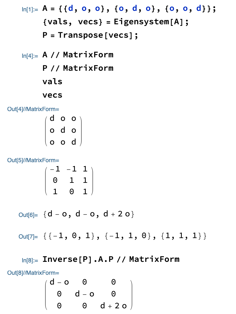
Demonstration in Mathematica

Demonstration in Jupyter-notebook with sympy

Reference

• G. Strang, Linear algebra and its applications, 4th Ed. (Thomson, Brooks/Cole, Belmont, CA, 2006) p.273.